• Menu
  About Myself Introduction Data Sources Data Visualization Exploratory Data Analysis ARMA/ARIMA/SARIMA Models Financial Time Series Models (ARCH/GARCH) Deep Learning for TS Conclusions

ARMA/ARIMA/SARIMA Models

• Check Stationarity of Original Data

	Solar Power	Gas
ACF Plots	(Click to see a larger view.)	(Click to see a larger view.)
ADF Tests	(Click to see a larger view.)	(Click to see a larger view.)

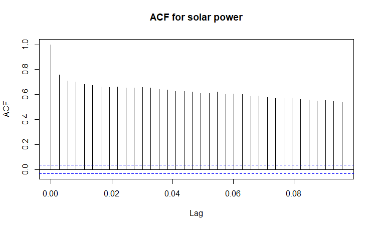
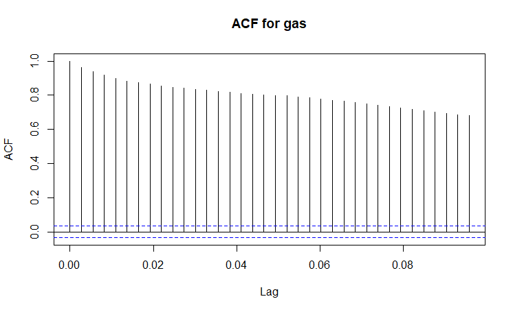
The series for both solar power and gas are not stationary, since ACF plots show strong correlations between observations. ADF tests give statistically significant results for both solar power and gas at 0.05 significance level, indicating they are stationary. However, apparently they are not. It seems that alpha-error happens.

• Check Stationarity of Differenced Data

	Solar Power	Gas
Time Series Plots	(Click to see a larger view.)	(Click to see a larger view.)
ADF Tests	(Click to see a larger view.)	(Click to see a larger view.)

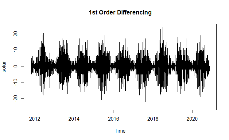
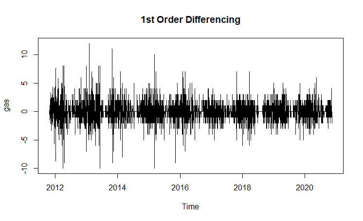
The series for both solar power and gas are stationary since the time series plots show constant mean. After differencing process, the p-values of ADF tests are less than 0.05, which give significant results, indicating that the series for both solar power and gas are now statistically stationary.

• Decide the order (p,d,q) of ARIMA model

	Solar Power	Gas
ACF Plots	(Click to see a larger view.)	(Click to see a larger view.)
PACF Plots	(Click to see a larger view.)	(Click to see a larger view.)

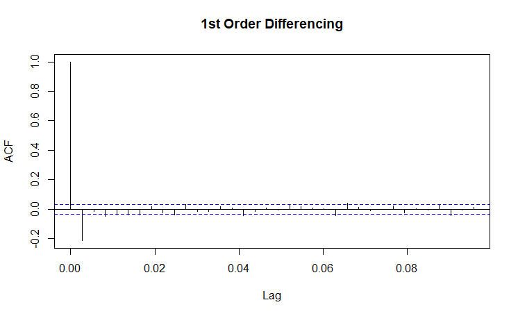
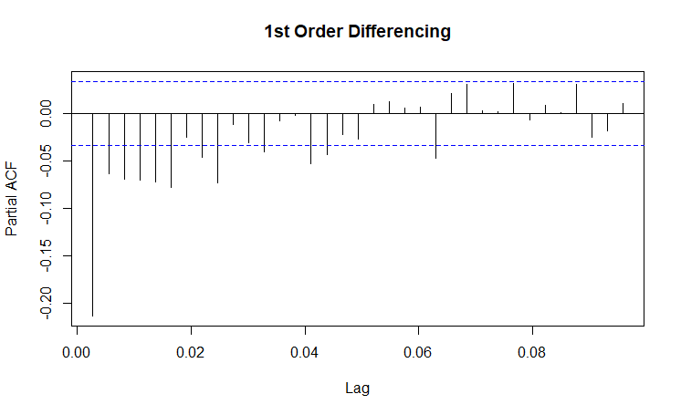
For solar power data, d = 1 since the series is stationary after 1st order differencing. From the ACF plot, max q = 3 since a cutoff happens after lag 3. From the PACF plot, p = 0 since there is a exponentially decaying in the PACF plot.

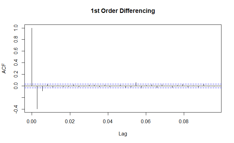
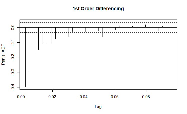
For gas data, d = 1 since the series is stationary after 1st order differencing. From the ACF plot, max q = 2 since a cutoff happens after lag 2. From the PACF plot, max p = 6 since a cutoff happens after lag 6.

• Fit ARIMA Models

	Solar Power	Gas
AIC & BIC	(Click to see a larger view.)	(Click to see a larger view.)
Coefficients	(Click to see a larger view.)	(Click to see a larger view.)
Equations	(Click to see a larger view.)	(Click to see a larger view.)

For solar power data, the best ARIMA model is ARIMA(1,1,1) according to the lowest BIC. For gas data, the best ARIMA model is ARIMA(2,1,1) according to the lowest BIC.

• Model Diagnostic

Solar Power	Gas
(Click to see a larger view.)	(Click to see a larger view.)

The residual plots of the ARIMA model show that the standardized residuals look like random walk. Nearly all lines are within the boundaries in the ACF of residual plots. The Q-Q plot shows that the standard residuals are not actually normal distributed, but the p values for Ljung-Box statistics are large enough to not reject the null hypothesis, which means that the ARIMA models are perfect.

• Forecast

Solar Power	Gas
(Click to see a larger view.)	(Click to see a larger view.)

From the forecast, the amount of daily power production of solar panels and used gas are both going constant in the future 100 days.

• Benchmark Methods

	Solar Power	Gas
Mean	(Click to see a larger view.)	(Click to see a larger view.)
Naive	(Click to see a larger view.)	(Click to see a larger view.)
Seasonal Naive	(Click to see a larger view.)	(Click to see a larger view.)
Random Walk	(Click to see a larger view.)	(Click to see a larger view.)

The ARIMA models with naive method and random walk with drift are the same.

• Fit SARIMA Models

	Solar Power	Gas
ACF Plots	(Click to see a larger view.)	(Click to see a larger view.)
PACF Plots	(Click to see a larger view.)	(Click to see a larger view.)
Auto Arima	(Click to see a larger view.)	(Click to see a larger view.)
Residuals	(Click to see a larger view.)	(Click to see a larger view.)
Forecast	(Click to see a larger view.)	(Click to see a larger view.)
Benchmark Methods	(Click to see a larger view.)	(Click to see a larger view.)
Cross Validation	(Click to see a larger view.)	(Click to see a larger view.)

The best SARIMA model using auto.arima() for solar power data is ARIMA(4,0,0)(0,1,0)[365], and the best SARIMA model using auto.arima() for gas data is ARIMA(3,0,0)(0,1,0)[365]. The forecasts using SARIMA models are much better than ARIMA models. Compared with all benchmark methods, the forecast using seasonal naive method is the best.