• Menu
  About Myself Introduction Data Sources Data Visualization Exploratory Data Analysis ARMA/ARIMA/SARIMA Models Financial Time Series Models (ARCH/GARCH) Deep Learning for TS Conclusions

Exploratory Data Analysis

• Time Series Plots

Solar Power	Gas
(Click to see a larger view.)	(Click to see a larger view.)

Both daily solar power production of solar panels and daily used gas show strong seasonality, with strong cyclic behavior with a period of about one year. However, the peaks and nadirs of daily used gas are opposite to solar power production. It seems there were more solar power production in summers and less in winters, which means that warm days are likely to produce more solar power. On the contrary, more gas were used in winters, mainly because people used more gas to produce heat and keep warm in winters.

• Lag Plots

Solar Power	Gas
(Click to see a larger view.)	(Click to see a larger view.)

The lag plot of gas shows a more strongly positive relationship than solar power, reflecting stronger seasonality in the gas data.

• Decomposition Plots

	Multiplicative	Additive
Solar Power	(Click to see a larger view.)	(Click to see a larger view.)
Gas	(Click to see a larger view.)	(Click to see a larger view.)

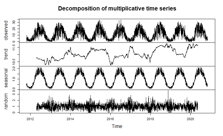
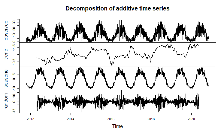
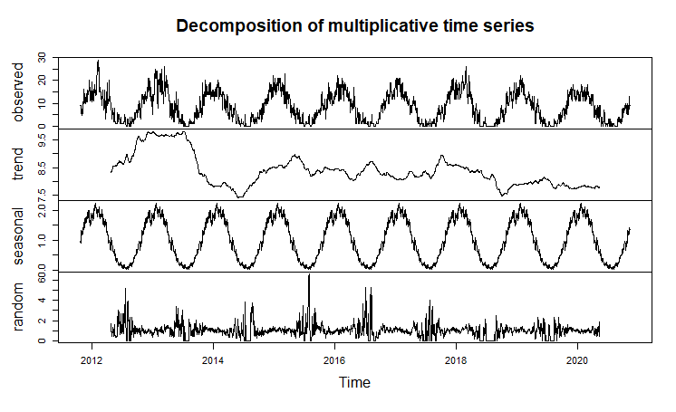
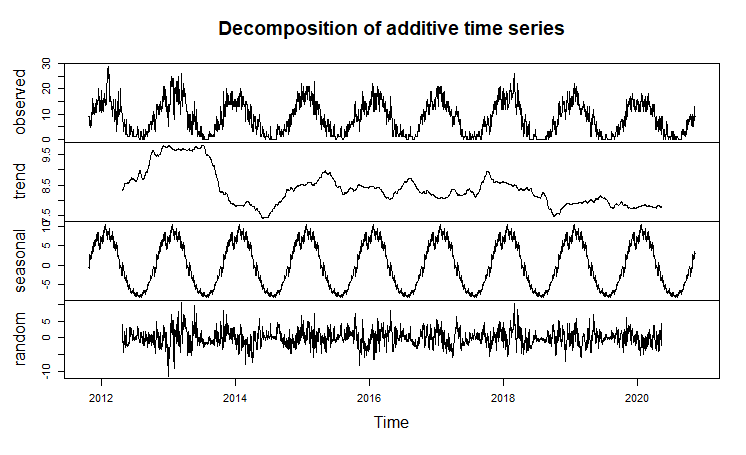
Decomposing method is applied to look deeper into the components of the series for solar power and gas. From the plots, the trend and seasonal components are clearly discovered. After detrending the data, the seasonality looks much more steady. The series for both solar power and gas are additive.

• ACF & PACF Plots

	ACF Plots	PACF Plots
Solar Power	(Click to see a larger view.)	(Click to see a larger view.)
Gas	(Click to see a larger view.)	(Click to see a larger view.)

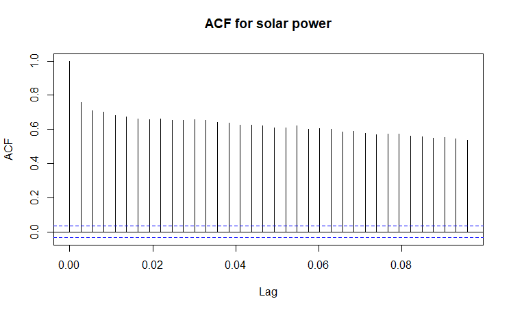
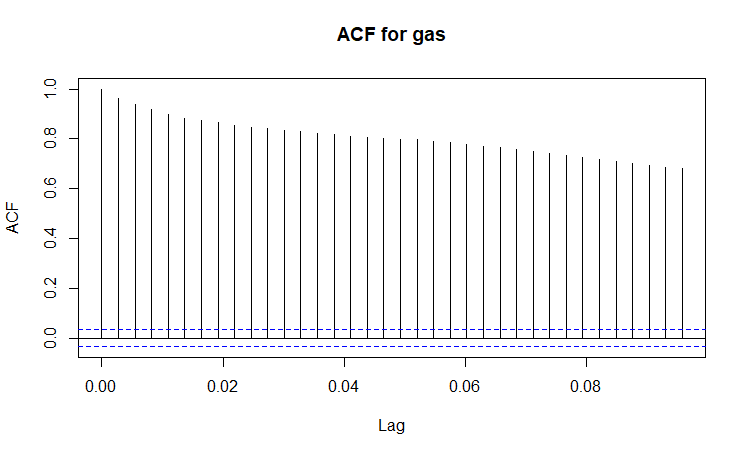
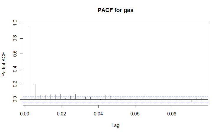
The ACF plots show strong correlations between an observation and another observation for all lags. The PACF plots show strong correlations between an observation and its lag when lag is less than 0.05. The ACF and PACF plots show that the series for both solar power and gas are not stationary.

• Detrend Data (Differencing)

	Time Series Plots	ACF Plots
Solar Power	(Click to see a larger view.)	(Click to see a larger view.)
Gas	(Click to see a larger view.)	(Click to see a larger view.)

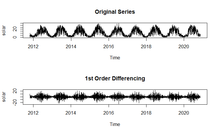
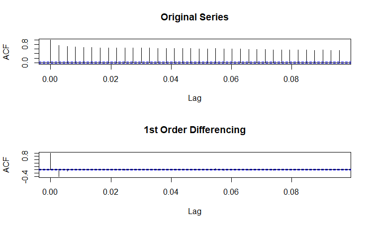
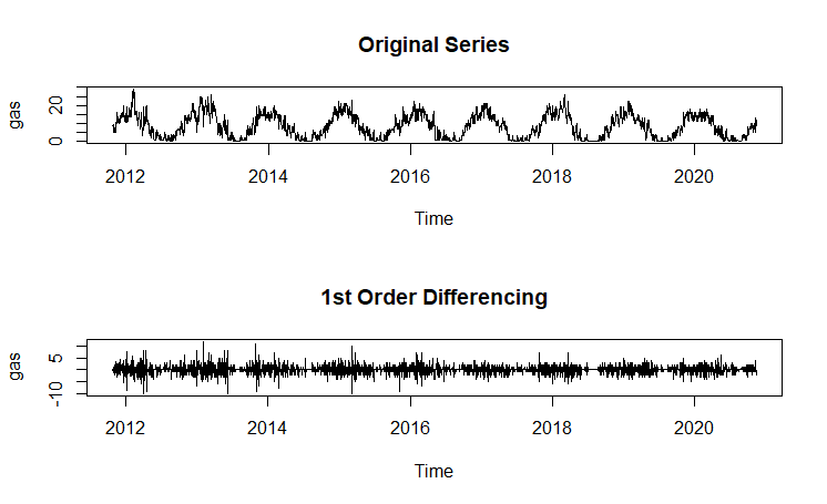
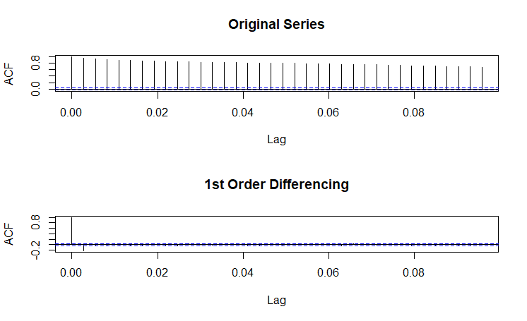
Differencing is used to remove trend from the solar power and gas data. The ACF plots show strong auto correlations between observations when lag equals to first two lags, then a sharp decline to low correlations beyond that. From the time series plots and the ACF plots, the series for both solar power and gas are stationary after the differencing process.

• Augmented Dickey-Fuller Test

Solar Power	Gas
(Click to see a larger view.)	(Click to see a larger view.)

After the differencing process, the p-values of ADF tests are less than 0.05, which give significant results, indicating that the series for both solar power and gas are now statistically stationary.

• Moving Average Smoothing

	Solar Power	Gas
window = 5	(Click to see a larger view.)	(Click to see a larger view.)
window = 10	(Click to see a larger view.)	(Click to see a larger view.)
window = 50	(Click to see a larger view.)	(Click to see a larger view.)
window = 100	(Click to see a larger view.)	(Click to see a larger view.)
window = 200	(Click to see a larger view.)	(Click to see a larger view.)

When the window is getting larger, the method considers a longer period, making the cyclic behavior clearer but the detail of each data point is blurred. The seasonality cannot be seen from the last two smoothings.